Features of PanDiffusion
Overall Design
-
Time evolution of composition profile, phase volume fraction, and phase composition.
-
Multiple selections of thermal history, boundary condition and geometry.
-
Applications including particle dissolution, carburization, decarburization, homogenization, phase transformation, and diffusion couple.
Kinetic Model
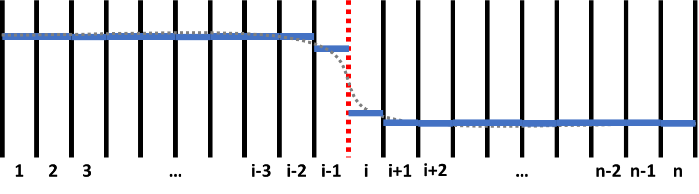
Figure 1 shows a schematic plot of a composition profile in a diffusion couple. In the simulation, the sample is divided by grids with equal width. The numbers, 1, 2, 3, …, n, indicate grid id. The solid black and dashed red lines means inter-grid interface. What is more, the red dashed line between (i-1)-th and i-th grids indicates the position of a sharp interface of this diffusion couple. Inter-grid flux is calculated following Fick’s first law. The interface between different phases have different special treatments such as “moving-boundary” model and " plain" model. Moving-boundary model is especially required for simulating Solid-Liquid interfaces. An example for simulating the diffusion between solid Al and liquid Zn is provide in the example folder (See AlZn_Solid_Liquid_diffusion_couple.pbfx). Composition of each grid, which is indicated by solid blue line in Figure 1, is calculated following Fick’s second law. The discrete composition profile represents a continuous composition profile of gray dashed line. Chemical potential, mobility, phase equilibrium and related properties are updated for each grid after calculating the composition.
Flux Model
The evolution of each grid’s composition is controlled by the inter-grid flux which is calculated based on absolute reaction rate theory [1941Gla]. At the lattice-fixed frame of reference, the flux is:

|
(1) |
Where  is the flux of k-th element between the grid i and the grid i+1.
  is effective mobility, R is the gas constant, T is temperature in Kelvin,
  is molar volume,
  is the thickness of grid interface and in most cases calculated as average grid size,
  and
and  are molar fraction of k-th element at the grid i and the grid i+1,
  is the chemical potential difference of k-th element between the grid i and the grid i+1. The sinh is the hyperbolic sine function. For convenience of calculation, a composition profile is observed at a volume-fixed frame of reference, and the flux of substitute element is transformed to
  .
.
Then the amount of k-th element ( ) of each grid can be updated according Fick’s 2nd law:

|
(2) |
Where unit normal vectors point outward from the grid.
[1941Gla] S. Glasstone et al., “The theory of rate processes”, New York, NY: McGraw-Hill; 1941.